What are the types of Financial Models? Explained with Examples

Financial models are crucial tools used by businesses, financial analysts, investors, and other stakeholders to forecast a company’s future financial performance based on historical data, current market conditions, and various assumptions. There are various types of financial models that can be used to forecast and value a company. These models serve several purposes, from evaluating the viability of a new project to assessing potential investment opportunities.

Types of Financial Models

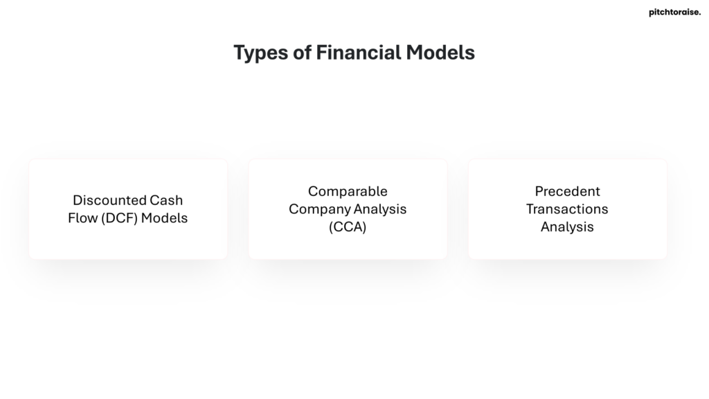
Most financial models fall into one of the following categories:

Discounted Cash Flow (DCF) Model

• Estimates the value of an investment based on its expected future cash flows.
• Utilizes the concept of the time value of money to discount future cash flows to their present value.

Comparable Company Analysis (CCA)

• Values a company based on the valuation metrics of similar companies in the industry.
• Commonly uses multiples like Price/Earnings (P/E) and Enterprise Value/EBITDA.

Precedent Transactions Analysis

• Involves valuing a company by examining past transactions of similar businesses.
• Uses valuation multiples from previous M&A activities to benchmark the target company.

Applications of Financial Models

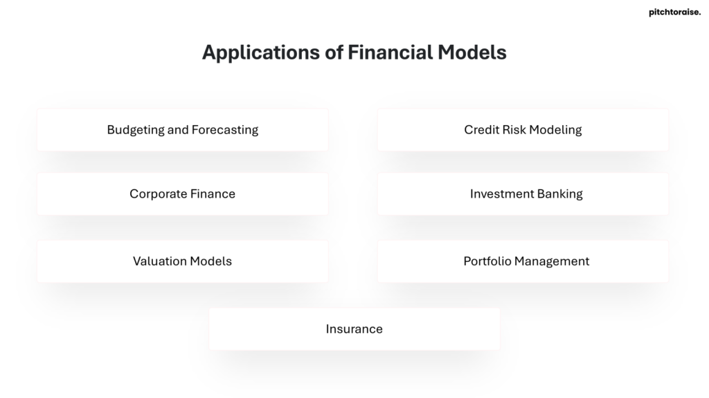
1. Budgeting and Forecasting:
   • Used by companies to create detailed budgets and forecasts, projecting future revenues, expenses, and cash flow.
2. Corporate Finance:
   • Employed in assessing mergers and acquisitions, capital raising, and other corporate finance activities.
3. Valuation Models:
   • Utilized by analysts to estimate the value of companies and securities, employing methods like Discounted Cash Flow (DCF) and Comparable Company Analysis.
4. Credit Risk Modeling:
   • Banks and financial institutions use these models to evaluate the creditworthiness of borrowers, predicting potential default risks.
5. Investment Banking:
   • Essential for deal structuring, pricing, and evaluating the financial impact of transactions.
6. Portfolio Management:
   • Used by portfolio managers to assess the risk and return profiles of investment portfolios, optimizing asset allocations.
7. Insurance:
   • Insurers use financial models to determine premiums, reserves, and to analyze risk scenarios.

Advanced Applications

• Algorithmic Trading:
  • Financial models are integral in developing algorithms for high-frequency trading, enhancing trading strategies.
• Economic Scenario Analysis:
  • Used by economists and policymakers to simulate the impact of different economic policies and external shocks on the economy.

Financial models serve as vital tools across various sectors, underpinning a wide array of financial activities and strategic decisions. By transforming data into actionable insights, these models enhance precision, foresight, and strategic agility.

Basic Financial Models Overview

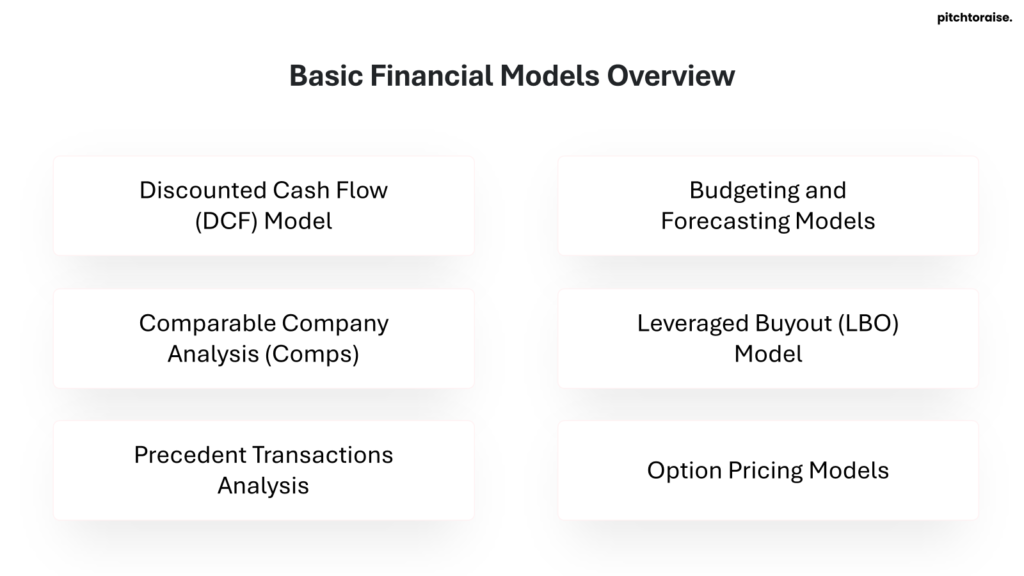
Financial models serve as crucial tools for various financial analysis tasks, offering structured approaches to evaluate performance, forecast outcomes, and assess risks. Below is an overview of some basic financial models commonly utilized:

1. Discounted Cash Flow (DCF) Model

The DCF model estimates the value of an investment based on its expected future cash flows. These cash flows are discounted back to their present value using a discount rate, usually the weighted average cost of capital (WACC).

• Advantages:
  • Provides a detailed outlook on future cash flows
  • Useful for investment appraisals and valuations
• Disadvantages:
  • Highly sensitive to input assumptions
  • Can be complex to develop

2. Comparable Company Analysis (Comps)

Comparable Company Analysis involves evaluating similar businesses to derive valuation metrics for a subject company. Metrics such as P/E ratios, EV/EBITDA, and P/B ratios are commonly used.

• Advantages:
  • Easy to understand and implement
  • Provides a range of valuation multiples
• Disadvantages:
  • Subject to market fluctuations and comparability issues
  • Relies on the availability and accuracy of data

3. Precedent Transactions Analysis

This model assesses past transactions of similar companies to establish valuation benchmarks. It uses multiples derived from acquisitive transactions.

• Advantages:
  • Reflects actual market premiums and discounts
  • Effective for merger and acquisition valuation
• Disadvantages:
  • Limited by the availability of comparable transactions
  • May not account for unique factors of individual deals

4. Budgeting and Forecasting Models

These models assist organizations in planning and projecting future financial performance. They usually involve detailed revenue, expense, and capital expenditure forecasts.

• Advantages:
  • Enhances financial planning and management
  • Provides benchmarks for performance evaluation
• Disadvantages:
  • Time-consuming to develop and maintain
  • May require frequent updates due to changes in assumptions

5. Leveraged Buyout (LBO) Model

An LBO model evaluates the acquisition of a company using a significant amount of borrowed funds. It projects the company’s ability to service debt and generate returns on equity.

• Advantages:
  • High potential for high returns due to leverage
  • Effective for assessing buyout feasibility
• Disadvantages:
  • High-risk due to leverage
  • Complex to build and requires robust assumptions

6. Option Pricing Models

Option pricing models, like the Black-Scholes model, are used to estimate the fair value of options based on factors like volatility, time to expiration, and strike price.

• Advantages:
  • Essential for derivatives trading and risk management
  • Provides insights into market expectations
• Disadvantages:
  • Complex mathematical underpinnings
  • Requires accurate inputs for reliability

Each of these models offers unique strengths and limitations, catering to specific use cases in financial analysis and valuation. Proficiency in these models equips financial professionals with the tools necessary to make informed decisions.

Advanced Financial Models Overview

Advanced financial models amplify basic modeling techniques by incorporating complex variables and environments. These models often leverage sophisticated algorithms and large datasets to forecast outcomes and assist in strategic decision-making. Advanced financial models are indispensable tools for financial analysts, risk managers, and executives seeking a comprehensive understanding of financial dynamics.

Types of Advanced Financial Models

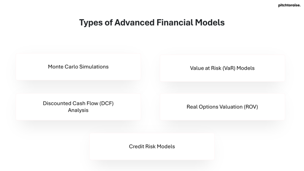
1. Monte Carlo Simulations
   • Monte Carlo simulations use random sampling to solve problems that might be deterministic in nature. They are used to model the probability of different outcomes in a process that cannot easily be predicted due to the intervention of random variables.
2. Value at Risk (VaR) Models
   • Value at Risk (VaR) is a statistical technique used to measure and quantify the level of financial risk within a firm or investment portfolio over a specific time frame. This model estimates the maximum potential loss with a given degree of confidence.
3. Discounted Cash Flow (DCF) Analysis
   • DCF analysis is a valuation method used to estimate the value of an investment based on its expected future cash flows. This model discounts future cash flows back to their present value to provide a clear picture of the investment’s worth.
4. Real Options Valuation (ROV)
   • Real options valuation applies financial options theory to investment decisions, providing a framework to value flexibility in projects, such as the ability to defer, expand, or abandon investments.
5. Credit Risk Models
   • Credit risk models assess the likelihood that borrowers will default on their obligations. These models combine borrower-specific data with macroeconomic conditions to predict potential losses and inform lending decisions.

Applications of Advanced Financial Models

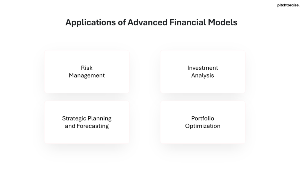
1. Risk Management
   • Advanced financial models provide robust frameworks for identifying and mitigating risks. For example, VaR models help in the management of market risk and credit risk, ensuring that firms maintain adequate capital reserves.
2. Strategic Planning and Forecasting
   • Companies utilize these models to develop long-term strategic plans and financial forecasts. Monte Carlo simulations, for instance, assist in understanding the potential variability in future cash flows under different scenarios.
3. Investment Analysis
   • Advanced models like DCF and ROV play a crucial role in investment decision-making processes. They aid in determining the potential return on investments and the viability of capital projects.
4. Portfolio Optimization
   • By employing techniques such as mean-variance optimization, financial firms can construct portfolios that maximize returns for a given level of risk, balancing potential gains against potential losses.

Key Considerations

• Data Quality
  • High-quality, reliable data is essential for the accuracy of any advanced financial model.
• Model Validation
  • Regular validation and back-testing are crucial to ensure that the models accurately represent real-world dynamics.
• Computational Resources
  • Advanced models often require significant computational power and resources, particularly for simulations and large-scale data analysis.

Advanced financial models are critical for organizations striving to navigate complex financial landscapes, mitigate risks, and seize strategic opportunities. They offer a deeper, more nuanced understanding of financial markets and investment decisions, paving the way for more informed and effective financial management.

Capital Budgeting Models: Real-World Example

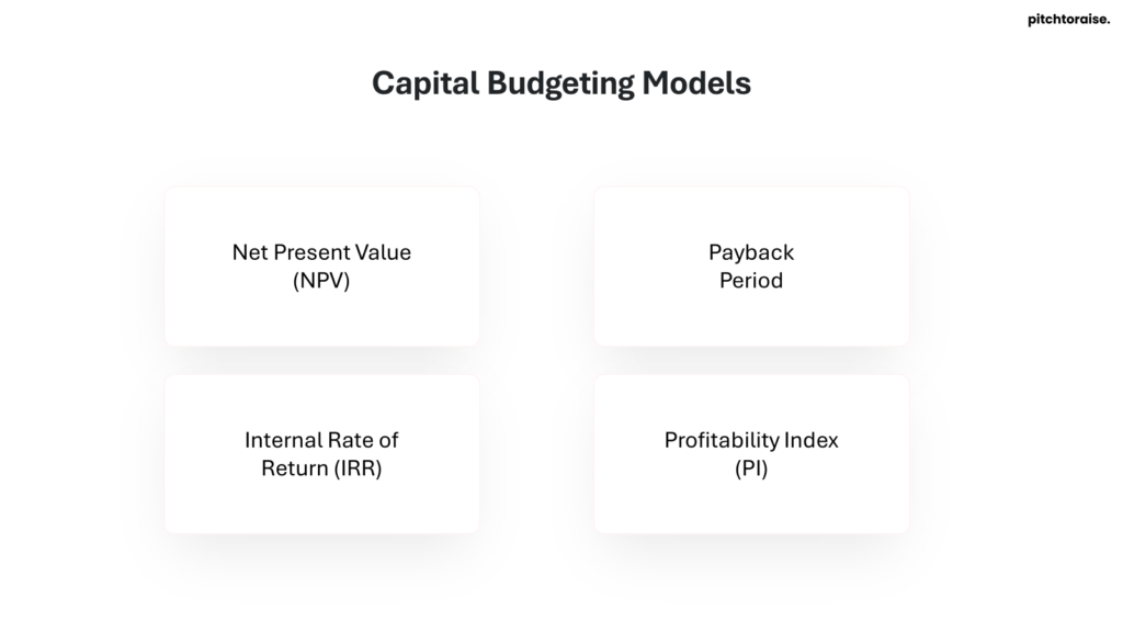
Capital budgeting models are essential for companies when evaluating large-scale investment projects. For instance, a global tech firm considering the development of a new data center may utilize various capital budgeting models to determine project feasibility and profitability.

Net Present Value (NPV)

The tech firm starts by calculating the Net Present Value (NPV) to assess the expected net cash flows from the data center project over its life span. The steps include:

• Estimating future cash flows.
• Determining the discount rate, often the firm’s cost of capital.
• Discounting the estimated cash flows to their present value.
• Summing these present values to find the NPV.

The formula used is:

[ \text{NPV} = \sum \left( \dfrac{R_t}{(1 + i)^t} \right) – C_o ]

Where:

• ( R_t ) is the net cash inflow during the period ( t ),
• ( i ) is the discount rate,
• ( t ) is the number of time periods, and
• ( C_o ) is the initial investment.

Internal Rate of Return (IRR)

Next, the firm calculates the Internal Rate of Return (IRR) to understand the return rate at which the NPV of all cash flows equals zero. This helps in comparing the profitability of the new data center with other investment options.

Payback Period

The tech firm also uses the Payback Period model to estimate the time required to recover the initial investment from the project’s cash inflows. This is crucial for understanding the project’s liquidity risk.

Profitability Index (PI)

Further, the Profitability Index (PI) is calculated by dividing the present value of future cash flows by the initial investment. A PI greater than 1 indicates that the project is considered profitable.

Practical Application Example

Consider a tech firm that projects an initial $10 million investment in a data center. The estimated cash inflows over five years are:

1. Year 1: $2 million
2. Year 2: $3 million
3. Year 3: $3 million
4. Year 4: $4 million
5. Year 5: $5 million

Assuming a 10% discount rate:

• The NPV calculation might show a positive value, indicating investment viability.
• The IRR might be found to be 15%, suggesting a good return.
• The Payback Period might be around 3 years, giving a quick insight into liquidity.
• The PI might be 1.2, reinforcing project profitability.

Accurate capital budgeting models provide the tech firm with critical insights to make well-informed decisions on capital investments.

Discounted Cash Flow (DCF) Models: Real-World Example

Discounted Cash Flow (DCF) models are widely used in finance for valuing a company, project, or asset based on its expected future cash flows. This valuation method is essential in making informed investment decisions. The example below demonstrates the application of a DCF model to evaluate a hypothetical company’s stock.

Step-by-Step DCF Analysis

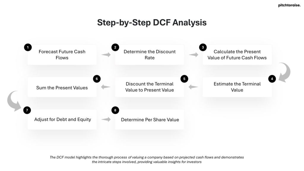
1. Forecast Future Cash Flows

A company’s free cash flow (FCF) projections over a forecast period, typically 5-10 years, form the foundation of the DCF model.

• Year 1: $100,000
• Year 2: $120,000
• Year 3: $140,000
• Year 4: $160,000
• Year 5: $180,000

2. Determine the Discount Rate

The discount rate, often the Weighted Average Cost of Capital (WACC), reflects the riskiness of the cash flows.

• WACC: 10%

3. Calculate the Present Value of Future Cash Flows

Each cash flow is discounted back to its present value (PV).

PV = FCF / (1 + WACC)^t
Where t is the year number.

• Year 1 PV: $90,909
• Year 2 PV: $99,174
• Year 3 PV: $105,349
• Year 4 PV: $109,971
• Year 5 PV: $114,315

4. Estimate the Terminal Value

At the end of the forecast period, assume a perpetuity growth rate (g) to estimate the terminal value (TV).

TV = FCF_last_year * (1 + g) / (WACC - g)

• Perpetuity Growth Rate (g): 3%
• Terminal Value: $2,828,235

5. Discount the Terminal Value to Present Value

Again, discount the terminal value.

• Terminal Value PV: $1,756,437

6. Sum the Present Values

Finally, add all present values together to get the total firm value.

• Total Firm Value: $2,925,156

7. Adjust for Debt and Equity

Subtract the company’s outstanding debt to derive the equity value.

• Debt: $500,000
• Equity Value: $2,425,156

8. Determine Per Share Value

Divide the equity value by the number of outstanding shares.

• Outstanding Shares: 100,000
• Per Share Value: $24.25

The DCF model highlights the thorough process of valuing a company based on projected cash flows and demonstrates the intricate steps involved, providing valuable insights for investors.

Comparative Company Analysis (CCA) Models: Real-World Example

Comparative Company Analysis (CCA) models are valuable tools in finance, allowing analysts to evaluate and compare the financial performance of different companies. Here is a real-world example of how CCA models are applied:

Example: Tech Industry Giants

In this example, analysts compare two major tech companies, Company A and Company B. These companies operate in the same industry and offer similar products and services, making them suitable candidates for comparative analysis.

Key Metrics Analyzed

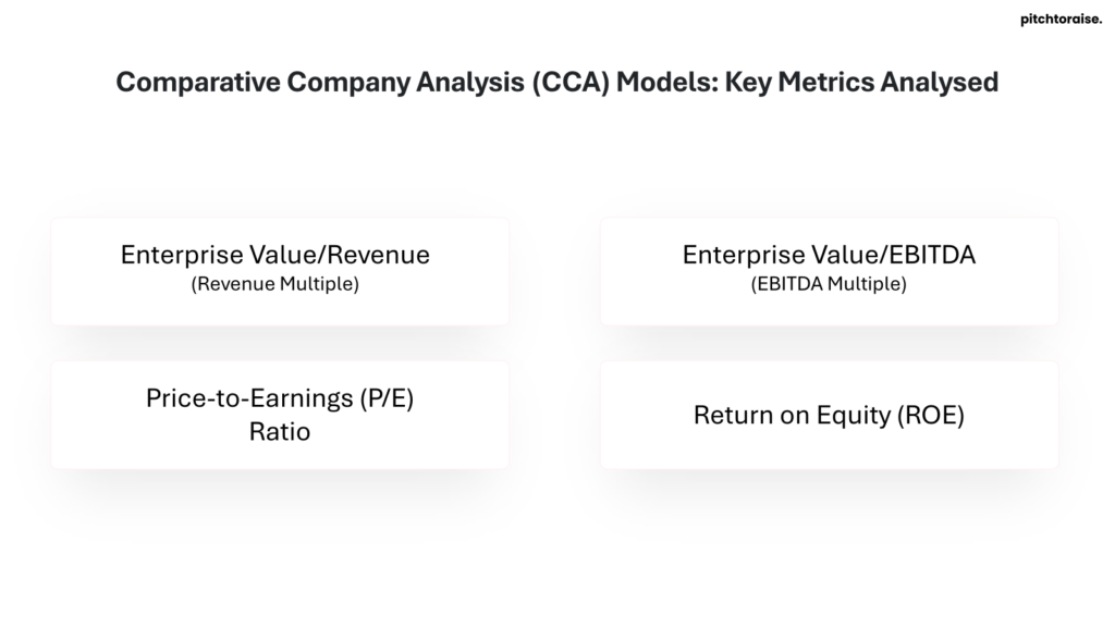
Analysts typically focus on various financial metrics to conduct a Comparative Company Analysis. Key metrics in this example include:

• Revenue Growth Rate: This metric indicates how quickly each company is increasing its sales over time.
• Earnings Before Interest, Taxes, Depreciation, and Amortization (EBITDA) Margin: EBITDA margin provides insights into the operational efficiency and profitability of the companies.
• Price-to-Earnings (P/E) Ratio: The P/E ratio helps assess the market valuation and investor expectations for each company.
• Return on Equity (ROE): ROE measures the profitability relative to shareholders’ equity, indicating how effectively each company is using equity financing.
• Debt-to-Equity Ratio: This ratio reveals the companies’ financial leverage and long-term solvency.

Data Collection

In a real-world scenario, analysts gather financial data from various sources:

• Annual Reports: Financial statements and management discussions from the companies’ annual reports provide detailed insight.
• Regulatory Filings: Reports filed with regulatory authorities, such as the SEC, offer reliable financial data.
• Market Data: Stock prices, market capitalization, and trading volumes are obtained from financial markets.
• Industry Reports: Analysis of industry trends and market conditions from reputed agencies.

Analytical Procedure

1. Normalization of Data: Analysts adjust financial figures to account for discrepancies in accounting practices, currency differences, or fiscal year variations.
2. Ratio Analysis: Calculation of key financial ratios for each company to facilitate comparability.
3. Benchmarking: Performance metrics of Company A and Company B are compared against industry averages and each other.
4. Qualitative Assessment: Factors such as management quality, business model resilience, and innovation potential are analyzed.

Findings and Interpretation

Through the CCA model, analysts find that:

• Company A has a higher revenue growth rate and better EBITDA margins but a slightly higher debt-to-equity ratio compared to Company B.
• Company B shows a more attractive P/E ratio, suggesting better market valuation relative to earnings, and a superior ROE, indicating effective equity utilization.

Conclusion

The CCA model’s findings help investors make informed decisions. In this case, some may favor Company A for its growth potential, while others might prefer Company B for its market valuation and profitability metrics.

Leveraged Buyout (LBO) Models: Real-World Example

Leveraged Buyout (LBO) models are essential tools in the financial sector, primarily used by private equity firms to assess the feasibility of acquiring companies through significant amounts of borrowed money. The real-world example of The Blackstone Group’s acquisition of Hilton Hotels in 2007 provides a comprehensive illustration of how LBO models operate.

In this transaction, Blackstone utilized approximately $20 billion of debt financing and $5.6 billion of equity to purchase Hilton Hotels for around $26 billion. This high debt-to-equity ratio is a staple feature of LBO models and plays a crucial role in their structure. The LBO model constructed for this acquisition would typically encompass the following key elements:

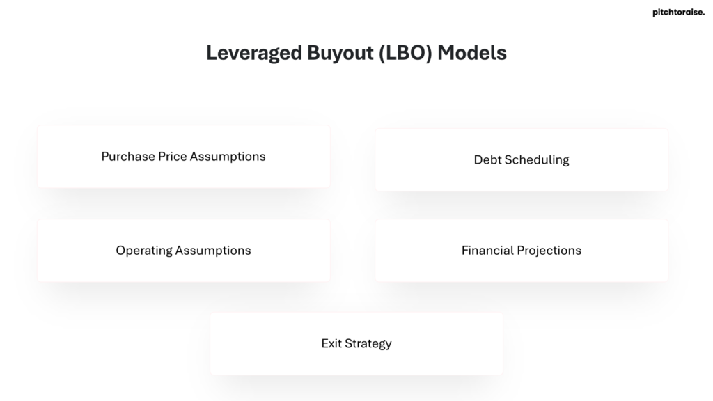
1. Purchase Price Assumptions:
   • The acquisition price of Hilton Hotels at $26 billion.
   • Breakdown of financing sources: $20 billion debt and $5.6 billion equity.
2. Operating Assumptions:
   • Projections for Hilton’s revenue growth, considering its market position and operational inefficiencies.
   • Cost Structure Analysis, focusing on fixed and variable costs to capitalize on potential synergies.
3. Debt Scheduling:
   • Detailed plan for servicing the $20 billion debt.
   • Various tranches of debt, categorized as senior debt, mezzanine debt, and subordinate debt.
   • Interest rates, repayment schedules, and covenants associated with each tranche.
4. Financial Projections:
   • Creation of Pro Forma Income Statements, Balance Sheets, and Cash Flow Statements.
   • Scenario Analysis, including base, upside, and downside scenarios, to gauge performance under different economic conditions.
5. Exit Strategy:
   • Time horizon for the exit, typically ranging from five to seven years.
   • Projected Exit Multiple on EBITDA to estimate the potential sale price of Hilton Hotels.
   • Internal Rate of Return (IRR) calculations to ensure the transaction meets the required return thresholds for Blackstone.

The Hilton acquisition exemplifies how LBO models are applied to real-world transactions, supporting decision-making through meticulous financial analysis. By involving extensive debt, equity infusions, and operational efficiency improvements, LBO models deliver a roadmap for transforming acquisitions into profitable ventures, often resulting in high returns for investors. This complexity underscores the importance of precise financial modeling in facilitating successful leveraged buyouts.

Merger and Acquisition (M&A) Models: Real-World Example

M&A models are essential for evaluating the financial implications of mergers and acquisitions, including valuation, synergies, financing, and post-acquisition performance. In practice, these models integrate various financial statements and predictive analytics to provide a comprehensive overview of potential deals.

Case Example: Disney’s Acquisition of 21st Century Fox (2019)

In 2019, The Walt Disney Company completed its $71 billion acquisition of 21st Century Fox. This significant M&A deal offers a practical example of how M&A models are utilized in the real world.

Objectives of the M&A Model

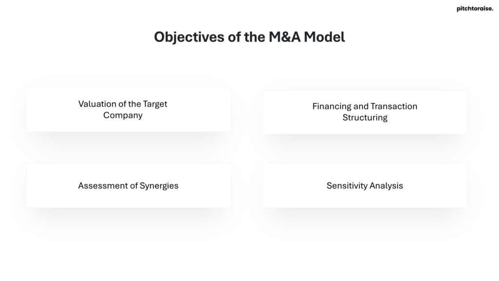
The primary objectives considered in this M&A model included:

1. Valuation of the Target Company:
   • Use of Discounted Cash Flow (DCF) analysis to determine 21st Century Fox’s intrinsic value.
   • Application of Comparable Company Analysis (CCA) and Precedent Transactions Analysis to benchmark valuation.
   • Consideration of potential revenue growth and cost-saving synergies.
2. Assessment of Synergies:
   • Identification of cost synergies from operational efficiencies.
   • Revenue synergies from cross-platform opportunities and enhanced content portfolios.
   • Calculation of Net Present Value (NPV) of synergistic benefits.
3. Financing and Transaction Structuring:
   • Analysis of optimal financing mix, including cash, stock, and debt.
   • Evaluation of the impact on Disney’s capital structure and credit rating.
   • Consideration of regulatory implications and the impact on shareholder value.
4. Sensitivity Analysis:
   • Examination of various scenarios such as fluctuations in revenue, cost synergies, and market conditions.
   • Stress testing to evaluate the robustness of the deal under different assumptions.
   • Risk analysis to foresee potential pitfalls and develop mitigation strategies.

Steps in Building the M&A Model

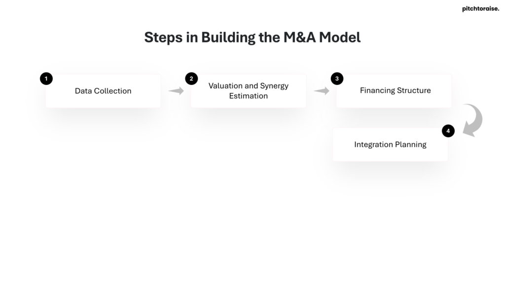
1. Data Collection:
   • Gather financial statements and market data for both Disney and 21st Century Fox.
   • Research industry trends, competitive landscape, and regulatory factors.
2. Valuation and Synergy Estimation:
   • Conduct detailed DCF analysis and comparable market analysis for 21st Century Fox.
   • Identify and quantify cost-saving and revenue-enhancing synergies.
3. Financing Structure:
   • Develop scenarios for different financing structures.
   • Analyze the impact on Disney’s balance sheet, earnings per share (EPS), and credit health.
4. Integration Planning:
   • Model the integration timeline and associated costs.
   • Measure potential disruptions and develop plans to mitigate integration risks.

Outcome and Impact

The M&A model provided Disney with a clear understanding of the financial benefits, risks, and strategic fit of acquiring 21st Century Fox. The deal significantly expanded Disney’s content library, enhancing its competitive position in the streaming market and leading to greater economies of scale.

Disney’s acquisition is a quintessential example demonstrating the importance and complexity of M&A modeling in making informed investment decisions.

Option Pricing Models: Real-World Example

Option pricing models serve as crucial tools in the financial sector, assisting traders, investors, and risk managers in determining the fair value of options. One well-known example is the Black-Scholes model, widely used for European options. Consider a real-world scenario involving a financial institution managing a portfolio of call options on XYZ Corporation’s stock. The primary objective is to price these options accurately to make informed trading and hedging decisions.

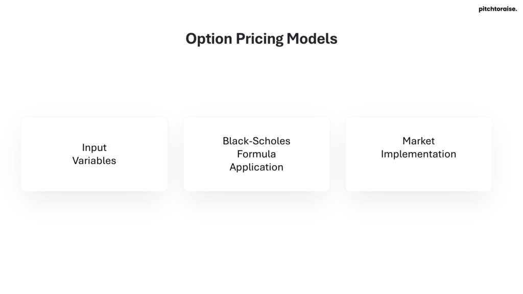
1. Input Variables:
   • Stock Price (S): Assume XYZ’s current stock price is $100.
   • Strike Price (K): The exercise price of the call option is set at $105.
   • Time to Maturity (T): The option expires in one year.
   • Risk-Free Rate (r): The current risk-free interest rate is 2%.
   • Volatility (σ): Historical data suggests a 20% annual volatility for XYZ stock.
2. Black-Scholes Formula Application:
   • The Black-Scholes model uses the following formula for a call option: [ C = S_0N(d_1) – Ke^{-rT}N(d_2) ] where: [ d_1 = \frac{\ln(S/K) + (r + \sigma^2/2)T}{\sigma\sqrt{T}} ] [ d_2 = d_1 – \sigma\sqrt{T} ]
   • Plugging in the variables: [ d_1 = \frac{\ln(100/105) + (0.02 + 0.2^2/2) \times 1}{0.2 \sqrt{1}} = 0.136 ] [ d_2 = 0.136 – 0.2 \sqrt{1} = -0.064 ]
   • Utilizing a standard normal distribution table: [ N(d_1) \approx 0.555 ] [ N(d_2) \approx 0.474 ]
   • Calculating the option price: [ C = 100 \times 0.555 – 105 e^{-0.02 \times 1} \times 0.474 \approx 7.53 ]
   • According to the Black-Scholes model, the fair value of the call option is approximately $7.53.
3. Market Implementation:
   • The financial institution uses the calculated option price to guide decisions:
     • Trading: Buying or selling options based on the model’s valuation.
     • Hedging: Managing risk through strategic positions.

Option pricing models like the Black-Scholes provide a standardized method to evaluate options, ensuring consistency and rationality in financial markets.

Sensitivity and Scenario Analysis: Real-World Example

In financial modeling, sensitivity and scenario analysis are instrumental in understanding the potential impact of different variables and events on a business’s financial performance. A real-world example is necessary to elucidate the practical application of these analyses.

Consider a multinational corporation planning to launch a new product line. The financial model developed for this project will include various assumptions, such as the cost of goods sold (COGS), sales price, market penetration rate, and fixed operating costs. Sensitivity analysis will evaluate how changes in these assumptions affect the company’s profitability.

Steps in Sensitivity Analysis

1. Identify Key Variables:
   • Sales Volume: Units sold per period.
   • Sales Price: Price per unit.
   • COGS: Cost per unit produced.
   • Operational Expenses: Fixed and variable costs.
2. Apply Variations:
   • Increase/decrease sales price by 5%, 10%, 15%.
   • Increase/decrease sales volume by 5%, 10%, 15%.
   • Increase/decrease COGS by 5%, 10%, 15%.
3. Evaluate Outcomes:
   • Calculate changes in Gross Profit Margin.
   • Assess impacts on Net Income.

Illustrative Example

Assume the corporation’s baseline model predicts:

• Sales Price per unit: $100
• COGS per unit: $60
• Sales Volume: 10,000 units
• Fixed Operational Expenses: $200,000

Performing sensitivity analysis on the sales price:

• Base Case: Revenue = $1,000,000, COGS = $600,000, Gross Profit = $400,000, Net Income = $200,000
• Scenario 1 (5% Increase in Sales Price): Revenue = $1,050,000, COGS = $600,000, Gross Profit = $450,000, Net Income = $250,000
• Scenario 2 (5% Decrease in Sales Price): Revenue = $950,000, COGS = $600,000, Gross Profit = $350,000, Net Income = $150,000

Scenario Analysis

Scenario analysis examines how different combinations of variables impact financial outcomes. Consider three potential future scenarios:

1. Optimistic Scenario: Higher market growth, increased demand.
   • Sales Volume: 12,000 units
   • Sales Price: $105/unit
2. Most Likely Scenario: Steady market conditions.
   • Sales Volume: 10,000 units
   • Sales Price: $100/unit
3. Pessimistic Scenario: Economic downturn, decreasing demand.
   • Sales Volume: 8,000 units
   • Sales Price: $95/unit

Financial projections under each scenario will guide strategic decisions. The optimistic scenario presents higher revenues and profits, suggesting aggressive marketing and sales strategies. Conversely, the pessimistic scenario identifies the need for cost-cutting measures and conservative budgeting.

By performing sensitivity and scenario analysis, the corporation gains comprehensive insights into the range of possible financial outcomes, enabling informed decision-making and risk management.

Common Challenges in Financial Modeling

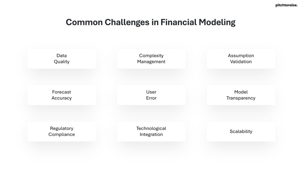
Financial modeling, despite being an essential tool for decision-making in finance, comes with a host of challenges. Professionals often grapple with several common issues that can hinder the accuracy and usefulness of their models.

• Data Quality: Ensuring the integrity of input data is crucial. Poor data quality, including inaccuracies, inconsistencies, and incompleteness, can lead to erroneous outputs. Reliable data sources and diligent verification are necessary to mitigate this issue.
• Complexity Management: Financial models often become complex as they account for numerous variables and scenarios. Striking a balance between comprehensive detail and usability is critical. Overly detailed models can be cumbersome, while oversimplified ones may miss critical factors.
• Assumption Validation: Models are often built on various assumptions which, if incorrect, can significantly skew results. Continuous validation and adjustments of these assumptions are essential. This requires domain knowledge and up-to-date information on market conditions.
• Forecast Accuracy: Predicting future financial performance involves a degree of uncertainty. Models must account for this by incorporating scenarios and sensitivity analyses. However, even with robust methodologies, forecasting remains an inexact science.
• User Error: Human error during data entry or formula configuration can impact model reliability. Implementing systematic checks, peer reviews, and automation where possible can reduce this risk.
• Model Transparency: Ensuring that a model is understandable to stakeholders is imperative. High transparency involves clear documentation, user-friendly design, and thorough auditing. Lack of transparency can result in mistrust and incorrect usage of the model.
• Regulatory Compliance: Financial models must comply with regulatory requirements, which can vary widely depending on the jurisdiction and industry. Keeping abreast of legal standards and incorporating them into the model is non-negotiable.
• Technological Integration: Leveraging advanced tools and software can enhance modeling capabilities but requires a steep learning curve and significant initial investments. Integrated systems must be user-friendly and adaptable to changes in financial environments.
• Scalability: As businesses grow, models need to scale accordingly. This scalability issue necessitates foresight during the initial model design phase to ensure it can handle increased complexity without significant rework.

By addressing these challenges systematically, financial professionals can enhance the reliability, accuracy, and utility of their financial models, making them more effective tools for strategic decision-making.

Best Practices in Financial Modeling

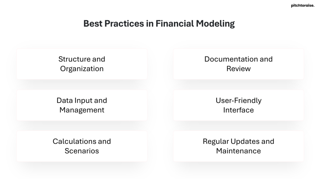
Financial modeling serves as a crucial tool in decision-making. Adopting best practices ensures accuracy, reliability, and efficiency.

Structure and Organization

• Consistent Formatting: Utilize a uniform structure for all models. Consistency in font, color codes, and layout improves readability.
• Clear Assumptions: Clearly delineate assumptions. Utilize a dedicated sheet for assumptions to avoid confusion.
• Modular Design: Design models in modular sections. This separation allows for easier updates and troubleshooting.

Data Input and Management

• Source Linking: Link data sources directly when possible. This practice ensures that data remains up-to-date and reduces manual errors.
• Data Segregation: Keep raw data separate from derived calculations. This separation prevents accidental alterations and maintains data integrity.
• Validation Checks: Integrate regular checks to validate data. Automated cross-checks can identify discrepancies early.

Calculations and Scenarios

• Dynamic Formulas: Use dynamic formulas to accommodate different scenarios. Avoid hardcoding values to ensure flexibility.
• Scenario Analysis: Incorporate scenario analysis for different outcomes. Utilize data tables or sensitivity analysis tools to demonstrate the impact of varying assumptions.
• Error Alerts: Include error-checking cells. Highlighting potential errors can prevent significant issues during analysis.

Documentation and Review

• Thorough Documentation: Document every element of the model. Well-documented models are easier to audit and transfer between users.
• Peer Review: Conduct regular peer reviews. A second set of eyes can catch errors and offer improvements.
• Version Control: Implement version control practices. Track changes to maintain a history of modifications.

User-Friendly Interface

• Intuitive Navigation: Design user-friendly models. Clear navigation aids users in finding relevant sections quickly.
• Input Prompts: Use input prompts or data validation to guide user input. This minimizes the risk of inadmissible data entries.

Regular Updates and Maintenance

• Scheduled Updates: Regularly update the model with new data. Consistent updates ensure that the model remains relevant.
• Maintenance Checks: Periodically review the model for necessary maintenance. This review includes updating outdated assumptions and removing obsolete data.

Adhering to these best practices ensures the creation of robust, reliable, and user-friendly financial models.

Tools and Software for Financial Modeling

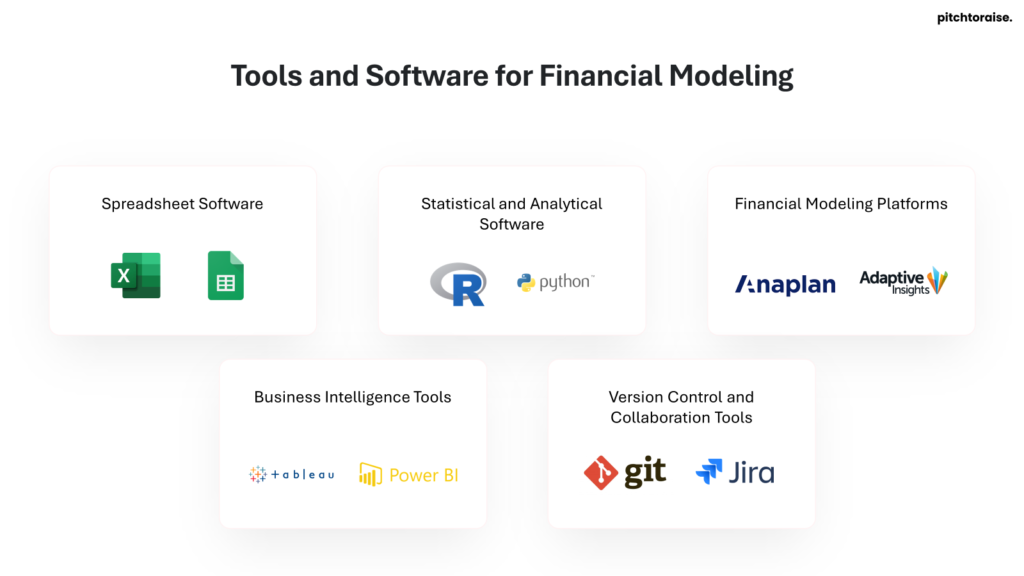
Financial modeling requires specialized tools and software to ensure accuracy and efficiency. Below is a list of commonly used tools:

• Microsoft Excel:
  • Description: Excel is one of the most widely used tools for financial modeling due to its flexibility, advanced computational capabilities, and broad recognition in the industry.
  • Use Cases: It is utilized for building detailed financial models, performing sensitivity analysis, scenario planning, and forecasting.
• Google Sheets:
  • Description: Google Sheets allows multiple users to collaborate in real-time, which enhances team-based financial modeling projects.
  • Use Cases: Ideal for simpler financial models, collaborative planning, and basic data analysis.
• Financial Modeling Software:
  • Examples:
    • Quantrix:
      • Description: Quantrix is tailored for advanced financial modeling with its multi-dimensional modeling capabilities.
      • Use Cases: Commonly used for high-complexity financial models, including those requiring multiple variables and in-depth scenario planning.
    • Adaptive Insights:
      • Description: Adaptive Insights offers cloud-based CPM software for budgeting, forecasting, and financial analysis.
      • Use Cases: Suitable for enterprise-level financial planning and analysis, particularly in large organizations aiming for comprehensive financial management.
• Automation Tools:
  • Examples:
    • Python with Pandas:
      • Description: Python, with its powerful Pandas library, is used for automating the extraction, transformation, and analysis of financial data.
      • Use Cases: Useful for building custom financial models, performing automated data manipulation, and complex financial analytics.
    • R:
      • Description: R is a statistical programming language known for its data analysis and visualization capabilities.
      • Use Cases: Employed in the creation of sophisticated financial models, statistical analysis, and visualization of financial data.
• Business Intelligence Tools:
  • Examples:
    • Tableau:
      • Description: Tableau provides robust data visualization capabilities for financial analysis.
      • Use Cases: Used to create interactive dashboards that offer insights into financial performance and trends.
    • Power BI:
      • Description: Microsoft’s Power BI offers advanced data analytics and visualization capabilities.
      • Use Cases: Ideal for integrating financial data from various sources and visualizing complex financial metrics.

By leveraging these tools, professionals can construct, analyze, and refine financial models with greater accuracy and efficiency.

Conclusion and Future Trends in Financial Modeling

The continuous evolution in the field of financial modeling is driven by several key factors, including advancements in technology, the increasing complexity of financial markets, and the growing demands for more sophisticated analytical tools. Financial models are consistently being refined to enhance accuracy and predictive capabilities, ensuring that they meet the dynamic needs of the industry.

Emerging Technologies in Financial Modeling

1. Artificial Intelligence and Machine Learning:
   • AI and ML algorithms are being increasingly utilized to identify patterns and predict future market behaviors.
   • These technologies facilitate the development of more adaptive and self-learning models that can process vast amounts of data in real-time.
2. Cloud Computing:
   • Cloud-based solutions enable the deployment of more accessible and scalable financial models.
   • Collaborative tools and platforms foster a more integrated approach to model development and application.
3. Blockchain and Distributed Ledger Technology:
   • Enhances transparency and security in financial transactions.
   • Aids in developing models that better manage decentralized financial data.

Trends in Model Applications

1. Increased Use of Predictive Analytics:
   • Financial institutions are leveraging predictive models to forecast market conditions and optimize investment strategies.
   • This use is expanding to areas such as risk management and fraud detection.
2. Enhanced Stress Testing and Scenario Analysis:
   • Regulators and organizations are emphasizing the need for robust stress testing capabilities.
   • This trend pushes for models that can simulate a wider range of potential economic conditions and impacts.
3. Integration with ESG Factors:
   • Models are increasingly incorporating Environmental, Social, and Governance (ESG) factors to assess the long-term sustainability of investments.
   • This integration reflects a broader shift toward responsible investing and heightened awareness of non-financial risks.

Challenges and Opportunities

1. Data Quality and Management:
   • Ensuring the integrity and accuracy of data remains a critical challenge.
   • There is an opportunity to develop more sophisticated data management frameworks and tools.
2. Regulatory Compliance:
   • Adapting to continually evolving regulatory requirements is essential.
   • Financial modeling must align with compliance standards, which presents ongoing refinement opportunities.
3. Skill Development:
   • The complexity of modern financial models requires a workforce proficient in quantitative analysis and advanced technologies.
   • Continuous education and training programs are vital to keep pace with advancements in the field.

The future of financial modeling lies in the convergence of traditional financial analysis with cutting-edge technologies. This synthesis promises more robust, accurate, and comprehensive models capable of addressing the multifaceted challenges and opportunities within the financial landscape.